

 558 お客様のコメント
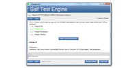

購入前に内容を確かめたい方のために、JPNTestでは2026年対応の77-727問題集無料サンプルをご提供しています。Microsoft Core Data Analysis, Manipulation, and Presentationに対応した35の問題の品質を、実際のPDFデモでご確認いただけます。
Microsoft 77-727 試験概要:
| 認定ベンダー: | Microsoft |
|---|---|
| 試験名: | Microsoft Excel 2016: Core Data Analysis, Manipulation, and Presentation |
| 試験番号: | 77-727 |
| 合格点: | 700/1000 |
| 試験形式: | パフォーマンスベースのタスク, プロジェクトベースの評価, 実機シミュレーション |
| 受験料: | $100 USD (地域によって異なります) |
| 関連資格: | Microsoft Office Specialist: Excel 2016 Expert (77-728) Microsoft Office Specialist: Excel 2016 |
| 試験時間: | 50-60 |
| 対応言語: | 中国語 (簡体字), 英語, ドイツ語, 日本語, フランス語, ポルトガル語, スペイン語 |
| 認定の有効期間: | 有効期限なし (MOS 2016 認定資格は原則として有効期限はありません) |
| 出題数: | 35-50 |
| 推奨トレーニング: | MOS Excel 2016 Expert 学習リソース Microsoft Learn - Excel 認定資格対策 |
| 受験申し込み: | Microsoft 資格情報 - MOS 認定 Microsoft 認定資格試験の登録 (Pearson VUE) |
| サンプル問題: | Microsoft 77-727 サンプル問題 |
| 受験方法: | オンライン監督試験または認定テストセンター (Pearson VUE) で受験可能 |
| 前提条件: | 必須の前提条件はありません。Microsoft Excel 2016 の高度な使用経験があることが推奨されます。 |
| 公式シラバスのURL: | https://learn.microsoft.com/credentials/certifications/mos-excel/ |
Microsoft 77-727 試験シラバストピック:
| セクション | 目標 |
|---|---|
| トピック 1: ブックの管理と共有 | - ブックのオプションと設定の管理 - 変更の追跡と管理 - ブックの共有と保護 |
| トピック 2: カスタムデータ書式とレイアウトの適用 | - ブックの構造とレイアウトの変更 - 条件付き書式の適用 - 高度な書式の適用 |
| トピック 3: 高度なグラフとテーブルの作成 | - テーブルと構造化データの操作 - グラフの書式設定と拡張 - グラフの作成と変更 |
| トピック 4: ピボットテーブルとツールを使用したデータ分析 | - ピボットテーブルの作成と管理 - ピボットグラフの作成 - データ分析ツールの使用 (What-If分析、予測) |
| トピック 5: 高度な数式と関数の作成 | - 論理関数と検索/行列関数の使用 - 数式の作成とトラブルシューティング - 文字列関数、日付関数、財務関数の適用 |
77-727試験のFAQ
「77-727」は、Microsoftが実施する「Microsoft Excel 2016: Core Data Analysis, Manipulation, and Presentation」の試験コードです。この試験に合格すると、「Microsoft Office Specialist (MOS) Excel 2016 Expert」の認定を取得できます。認定レベルはエキスパートに位置づけられています。関連する認定としては、Microsoft Office Specialist: Excel 2016 Expert (77-728)・Microsoft Office Specialist: Excel 2016などが挙げられます。JPNTestでは、77-727試験対策として35の練習問題をご用意しています。
77-727試験の出題数は35-50、制限時間は50-60です。限られた時間内で全問に取り組む必要があるため、1問にかけられる時間を常に意識し、難しい問題に長く留まりすぎないペース配分が求められます。本番で時間不足に慌てないよう、JPNTestのテストエンジンで制限時間つきの模擬試験に挑戦し、時間配分の感覚を体に覚えさせておくことをおすすめします。
77-727試験の合格ラインは700/1000、受験料は$100 USD (地域によって異なります)です。万が一不合格だった場合、再受験には改めて全額の受験料が必要になるため、費用面の負担も無視できません。受験前にJPNTestの35の練習問題で模擬試験に取り組み、安定して合格ラインを超えられることを確認してから本番に臨むと安心です。
必須の前提条件はありません。Microsoft Excel 2016 の高度な使用経験があることが推奨されます。
受験条件は変更される場合があります。最新かつ正確な情報は、Microsoftの公式ページで必ずご確認ください。
77-727試験は、以下の公式窓口からお申し込みいただけます。
なお、本試験の受験方式はオンライン監督試験または認定テストセンター (Pearson VUE) で受験可能です。
Microsoftでは77-727試験向けに、以下の公式トレーニングを用意しています。
公式トレーニングで知識の土台を固めたうえで、JPNTestの35の練習問題に取り組めば、理解度の確認と弱点の洗い出しを効率よく進められます。
はい、ご購入前にJPNTestの77-727問題集の無料サンプル(PDFデモ)をダウンロードして、問題の品質や形式をご確認いただけます。ご購入後は365日間の無料更新が付帯し、更新期間の終了後も50%割引で継続更新をご利用いただけるため、常に最新の出題傾向に沿った内容で学習を続けられます。
JPNTestでは「返金保証」制度をご用意しています。ご購入後60日以内に77-727試験を受験して不合格となった場合、全額返金をご申請いただけます。なお、ご購入後3日以内の受験や、ダウンロード後に実際の受験をしていない場合、無料資料や期限切れのご注文は対象外となり、受験者氏名とお支払い者氏名が一致している必要があります。ご申請の際は、受験票(enrollment slip)の写しと公式スコアレポート(Score Report)のPDFを試験後2日以内にご提出いただき、受理後7日以内に手続きが完了します。返金をご希望でない場合は、同等価値の試験資料2点を無料でお受け取りいただき、元の製品の更新サービスを継続する選択肢もございます。
また、ご購入いただいた製品はお支払い完了後すぐにダウンロードでき、メールでも1分以内にお届けします。2時間以内に届かない場合はカスタマーサポートまでご連絡ください。インストール可能なパソコンの台数に制限はありません。
77-727試験の出題範囲は、全部で5分野で構成されています。主な分野としては、「カスタムデータ書式とレイアウトの適用」、「ピボットテーブルとツールを使用したデータ分析」、「高度な数式と関数の作成」などが挙げられます。各分野の詳細なトピックと配点は、上記の試験大綱をご確認ください。JPNTestの77-727練習問題は、これらの出題分野を幅広くカバーしています。
Microsoft Core Data Analysis, Manipulation, and Presentation 認定 77-727 試験問題:
Project 1 of 7: Tailspin Toys
Overview
You recently opened an online toy store. You have sold products to 500 individual customers. You are
evaluating customer data and order data.


On the "Orders" worksheet, enter a formula in cell J2 that uses an Excel function to return the "OrderTotal"
value of the individual order that has the highest "OrderTotal" value.
See explanation below.
Explanation
1. Select the cell J2 where you want the highest "OrderTotal" value to be.
2. Type in the formula: =MAX(G1:G550).
References:
https://support.office.com/en-us/article/calculate-the-smallest-or-largest-number-in-a-range-45fe249f-96c3-443b
Project 4 of 7: Car Inventory
Overview
You manage the office of a used car business. You have been asked to prepare the inventory list for a big
annual sale.
Configure the "Car Inventory" worksheet so the column headings in row 9 appear on all printed pages.
See explanation below.
Explanation
1. On the "Car Inventory" worksheet, clickPrint Titlesfrom thePage Setupgroup, situated on thePage
Layouttab.
2. UnderPrint Titles, on theSheettab, type the reference of the row you want to reappear (row 9) in theRows to
repeat at topbox.
References:
https://support.office.com/en-us/article/Print-rows-with-column-headers-on-top-of-every-page-D3550133-F6A1-
Project 5 of 7: City Sports
Overview
The city events manager wants to analyze the enrollment changes over the past five years for various adult and
youth sports programs. You have been tasked to prepare tables for the analysis.

Unhide the "Summary" worksheet.
See explanation below.
Explanation
1. SelectFormatfrom theHometab then chooseHide and Unhidethen selectUnhide.
OR
1. Hold on the Ctrl button on the keyboard and choose all the worksheet tabs then choose theUnhideoption in
the right menu.
2. Click on the first worksheet tab, then hold down the Shift key on the keyboard as you click on the last
worksheet tab, then choose theUnhideoption.
OR
1. From theViewtab, clickCustom Viewsin theWorkbook Viewsgroup.
2. Click the "Summary" view which is hidden, then clickShow.
References:
https://www.isunshare.com/blog/hide-or-unhide-sheets-in-excel-2016/
Project 7 of 7: Farmers Market
Overview
You are the Director of a local farmers' market. You are creating and modifying charts for a report which
shows the amounts and variety of products sold during the season.

On the "Spring Sales" worksheet, add the title "New Products" to the column chart. Label the vertical axis
"Gross Sales" and the horizontal axis "Months".
See explanation below.
Explanation
1. Click on the title on the "Spring Sales" worksheet, then type "New Products".
2. You can edit theFontof the title from the mini-toolbar that appearsORfrom theHometab.
3. Click directly on either the x-axisory-axis in the chart OR click theChart Elementsbutton.
4. For editing the x-axis which is the horizontal category then type "Months".
5. Do the same to edit the y-axis which is the vertical category and type "Gross Sales".
6. You can further edit the text of the data in either of the axis as desired.
References:
https://www.dummies.com/software/microsoft-office/excel/how-to-edit-chart-titles-in-excel-2016/


 0
0
 0
0
 0
0
 0
0
